


MATLAB DSP Algorithms for Offline Signal Recovery and BER Counting
Tool Used: OptSim
MATLAB is often used for coherent receiver DSP algorithm research and development. In these application notes the signal after the photo-detector and the TIA is saved to a file and then processed offline with the MATLAB DSP algorithm scripts. This is the workflow typically adopted in the industry and OptSim and OptSim Circuit can seamlessly fit in.
All the MATLAB scripts are located in the directory named MATLAB included in the project directory. As a quick overview of this capability, consider a coherent system as described below: The data rate of the systems under consideration is 32 GBd and the number of symbol transmitted is 217 = 131072 bits. OptSim saves the signal directly to a MATLAB workspace file using the OptSim Compound Component for MATLAB (CCM).
The constant modulus algorithm (CMA) and Viterbi-Viterbi algorithm are used for polarization de-multiplexing and phase recovery. Once the signal is recovered the performance is estimated by doing BER counting.
The MATLAB DSP scripts return several types of information to the user. Figures 1 to 7 show the produced charts containing visual information about the characteristics of the signal before and after various stages of DSP processing. In addition the scripts perform BER counting on the recovered signal and return the BER for each individual bit stream as well as the final average BER.
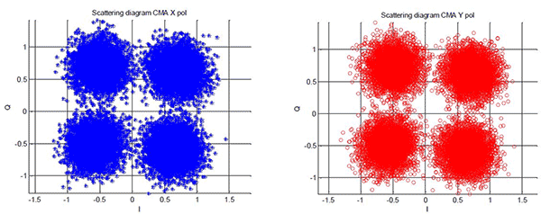
Figure 1. Scattering diagram after CMA for X and Y polarization

Figure 2. Phase error after Viterbi-Viterbi phase recovery for X and Y polarization
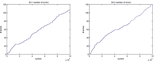
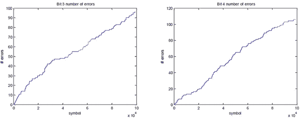
Figure 3. Total number of errors versus symbol number
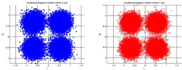
Figure 4. Scattering diagram after Viterbi-Viterbi for X and Y polarization

Figure 5. CloudPlot after Viterbi-Viterbi for X and Y polarization

Figure 6. FIR filter transfer function and impulse response
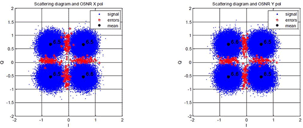
Figure 7. Signal and errors scattering diagram and OSNR for X and Y polarization