
Synopsys Cloud
Cloud native EDA tools & pre-optimized hardware platforms
Request a Free Trial →
The RSoft CAD offers a wide array of built-in refractive index profiles, but also allows custom index profiles to be defined using a mathematical expression in the User Profile Editor. These mathematical expressions can be functions of any combination of x, y, and/or z.
Custom index profiles are defined in the User Profile Editor window, which can be opened by clicking the Profiles… button in a segment properties dialog or via the Edit User Profiles button on the left CAD toolbar. Select a Source Type of “Expression” to define an index profile via a mathematical expression f(x', y', z'): for an arbitrary 3D user profile the index profile is expressed as n(x',y',z') = n0 + ∆nf(x',y',z'), where n0 is the background index, ∆n is the local index difference, and f(x’,y’,z’) is a profile function. The normalized coordinates x’,y’,and z’ are by default defined only within the component, and are defined as:
Where x,y, and z are the actual positions along the segment, and w,h, and l are the local width, height, and length of the segment. Therefore, the normalized coordinates are by default defined to vary between -1 and 1 for x’&y’, and between 0 and 1 for z’.
When using the User Profile Editor, it is necessary to convert the desired refractive index profile n(x,y,z) into a profile function f(x’,y’,z’) to be put into the editor. In the box below, we show how to re-write n(x,y,z) into f(x’,y’,z’).
The first step in converting n(x,y,z) → f(x',y',z') is to convert n(x,y,z) → n(x',y',z'). To do this, rewrite the equation for n(x,y,z) using the following coordinate transformations
To define the profile function f(x’,y’,z’) in terms of the normalized coordinates x’, y’, and z’, use the formulas
n(x',y',z') = n0 + ∆nf(x',y',z')
f(x',y',z') = (n(x',y',z') – n0)/∆n
Enter all coordinate variables in the User Profile Editor as x,y, and/or z; the CAD interprets the expression in the User Profile Editor based on the coordinate variables it finds as follows:
If z is present in the expression, the CAD will interpret z as z’.
If desired, for a structure with a circular-cross section a radially-dependent refractive index profile n(r,z) can be converted to a profile function f(r’,z’) which can be placed into the editor. In the box below, we show how to re-write n(r,z) into f(r’,z’).
The first step in converting n(r,z) → f(r',z') is to convert n(r,z) → n(r',z'). To do this, rewrite the equation for n(r,z) using the following coordinate transformations (keeping in mind that w=h for a structure with a circular cross-section)

To define a profile function in terms of the normalized coordinates r’&z’, use the formulas
n(r',z') = n0 + ∆nf(r',z')
f(r',z') = (n(r',z') – n0)/∆n
To express r’ in the User Profile Editor, use the variable x. If an expression in the User Profile Editor contains an x (but no y), the x is interpreted by the program as r’. If the expression contains both an x and a y, then x is interpreted as x’ and the y as y’.
To express z’ in the User Profile editor, use the variable z.
For more information about user profile conventions and normalized coordinates, please refer to sections 6.A.2 and 6.A.3 of the RSoft CAD manual.
As an example of using the User Profile Editor to define a custom profile, in the steps below we demonstrate how to use the User Profile Editor to define a 3D graded index optical fiber with the following refractive index profile.

Step 1: Define the fiber core
To draw the optical fiber (which has both a core and a cladding) in the RSoft CAD we will draw the core, and will later define the background to have the refractive index of the cladding. There is no need to draw the cladding directly; the core modes hardly see the cladding-air interface in an optical fiber, so directly drawing the cladding in the CAD can be excluded in order to save computational resources.
Using the Global Settings window, the Segment (In-Plane) drawing tool, and the Segment Properties window, draw the fiber core by drawing a straight segment with a circular cross-section.

In steps 2 & 3, we will define the optical fiber to have the following parameters.
| Variable | Value |
| α (fiber core radius) | 30µm |
| g (parameter that defines shape of profile) | 2 |
| N1 (nominal refractive index on-axis) | 1.45 |
| N2 (refractive index of cladding, taken to be homogeneous) | 1.44 |
| ∆ | |
| N(r) (nominal refractive index as a function of radius from fiber axis) | 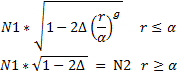 |
Step 2: Define appropriate variables in the Symbol table, and define the fiber cladding
Define ∆ (Delta), N1, N2, α (Alpha), and g in the Symbol table. For more information about the Symbol table, refer to section 3.C. of the RSoft CAD manual. Define the fiber cladding by setting the Background Index in the Global Settings window to N2. The user-defined refractive index profile n(r) will be created in step 3.
Step 3: Create the user-defined refractive index profile using an expression
Open the User Profile Editor window, which can be opened by clicking the Profiles… button in the segment properties dialog or via the Edit User Profiles button on the left CAD toolbar. Select a Source Type of “Expression” to define the index profile n(r) via a mathematical expression f(r’).
As described in the introduction, the profile function f(r’) to be used in the User Profile Editor can be derived from the desired refractive index profile n(r). In the box below, we derive f(r’) for this graded-fiber example.
n(r') = n0 + ∆nf(r')
f(r') = (n(r') – n0)/∆n
For a fiber with a circular cross-section of radius,
w = h = 2α

Thus, in normalized coordinates, the desired refractive index profile n(r') for the optical fiber core is
In the expression box, the normalized radial coordinate r’ is entered as x. If the expression contains both an x and a y coordinate, x&y are interpreted by the program as x’&y’. However, if the expression contains only a single x coordinate, x is interpreted as the normalized radial coordinate r’. Thus, f(r') should be entered in the User Profile Editor window as:
f(r') = (n(r') – n0)/∆n
n0 = N2
∆n = delta = N1-N2=0.01
n(r’) = N1*sqrt(1-2*Delta*(x)^g)
f(r') = (n(r') – n0)/∆n = (N1*sqrt(1-2*Delta*(x)^g)-N2)/delta
For more information about user profile conventions and normalized coordinates, please refer to sections 6.A.2 and 6.A.3 of the RSoft CAD manual. Insert the expression for f(r’) into the User Profile Editor. The number of points used to evaluate the expression is set via the X', Y', and/or Z' Points options. Fine resolutions can be useful to resolve rapidly changing functions or periodic functions. Once a profile has been defined, it can be viewed in the normalized coordinate system by clicking the Test button.

Step 4: Assign user-defined refractive index profile to structure, and view/check the structure.
Once a user profile has been defined, it can be assigned to a particular component via the Index Profile Type field in the segment properties dialog. The refractive index profile can be viewed using the Display Material Profile button in the left toolbar of the RSoft CAD. Right-clicking on any point in the contour plot will display a cut of the index profile contour map at that point, the cut taken can be vertical or horizontal depending on the cursor position.

It is also possible to interpret a user-defined profile absolutely, that is without refractive index or coordinate normalization, by enabling the “Absolute index in User Profile” option in the Global Index Generation Options window. In this case, the profile is interpreted absolutely but it is still translated from the coordinates defined in the expression/data file to the component center. If desired, a user profile can also be defined using a data file instead of an expression, please refer to section 6.A.3 of the RSoft CAD manual for further information.
We hope you found this tip helpful. If you have any questions, please contact us at rsoft_support@synopsys.com.
In April 2014, Microsoft stopped supporting Windows XP. In addition, usage of several other platforms currently supported by the RSoft products, such as Windows Vista, has drastically decreased. Therefore, RSoft products versioned 2013.12 are the last versions to officially support the following operating systems:
Please note that service releases for RSoft products versioned 2013.12 will also support Windows XP, Windows Vista, RHEL 4, and 32-bit versions of Windows and Linux.
Beginning in mid-2014, RSoft products beyond version 2013.12 will only officially support the following platforms:
We encourage you to migrate to 64-bit Windows or Linux computers, since official support for 32-bit versions of these operating systems has ended. If you have any questions, please contact rsoft_support@synopsys.com.
Graz, Austria
July 6-10, 2014
Enrico Ghillino1, Pablo Mena1,*, Vittorio Curri2, Andrea Carena2, Jigesh Patel1, Dwight Richards3, Rob Scarmozzino1
1Synopsys, Inc., 400 Executive Boulevard, Suite 100, Ossining, NY 10562, USA
2DET - Politecnico di Torino, Corso Duca degli Abruzzi, 24, 10129 Torino, Italy
3College of Staten Island, CUNY, 2800 Victory Boulevard, Staten Island, NY 10314, USA
*Tel: (914) 488-6269, Fax: (914) 488-6290, e-mail: pablo.mena@synopsys.com
ABSTRACT
Silicon photonic components are key enablers for low-cost, compact, and reduced power-consumption coherent transceivers. This paper discusses models used to analyze the performance of silicon photonic ring modulators in coherent links, and presents simulation results for 32- and 16-Gbaud PM-QPSK back-to-back transceivers incorporating these modulators in comparison with designs using LiNbO3 MZMs. While the penalty at 32 Gbaud is high, at 16 Gbaud the ring modulator performance approaches that of the MZM, with a sensitivity penalty of only 1.3 dB. Our results also show the strong temperature sensitivity of the ring modulator.


